
Most construction digital twins stop at dashboards. Real value begins when BIM becomes the semantic backbone for a live data pipeline. This post breaks down the full technical stack — IoT sensor ingestion via MQTT or Zerobus Ingest, BIM enrichment through IRI-based entity mapping and RDF triples, live twin state management, and low-latency operational serving via Lakebase. Built for engineers and solution architects, it covers architecture, tooling trade-offs, and data modeling patterns needed to build a construction digital twin that is genuinely operational. Part 2 shows how this pipeline changes real decisions on the ground.
The construction industry has long relied on periodic snapshots — blueprints, inspection reports, and site audits — to manage assets worth billions of dollars. The fundamental limitation of that approach is latency: a crack identified during a quarterly inspection could have been monitored continuously; an HVAC system drifting toward failure could have triggered a proactive response weeks earlier. A Digital Twin addresses this gap by maintaining a continuously updated virtual model of a physical asset, synchronized with real-world sensor data and operational events.
Building Information Modeling (BIM) provides the geometric and semantic foundation for this model. It is worth noting that modern BIM is not a passive data store — it already supports rule-based validation, clash detection, and phasing logic that structure how construction information is authored and coordinated. The step change delivered by a digital twin is connecting that structured model to live operational data, enabling the shift from design-time intelligence to runtime observability and decision support.
That integration, however, carries real complexity. Most construction programmes operate with established Common Data Environments (CDEs), ERP systems, and scheduling platforms that were not designed to exchange data at the frequency or fidelity that a digital twin demands. Bridging these systems requires deliberate data mapping, governance frameworks, and change management — not just a pipeline.
Digital twin initiatives in construction frequently stall or fail to deliver sustained value, and the causes are rarely technical in isolation. Data quality issues — inconsistent sensor calibration, incomplete as-built records, and schema mismatches — degrade twin fidelity over time. Mapping drift, where the relationship between physical assets and their twin identifiers loses accuracy as the site evolves, is a persistent operational risk. Without clear data ownership and governance, these problems compound quickly. This blog addresses the full stack: the architecture and tooling, and the data quality and governance practices that determine whether a twin remains reliable at scale.
A Digital Twin (DT) in construction mirrors its real-world counterpart in real time. Unlike a traditional BIM model that primarily captures static design intent and geometry, a digital twin captures the current operational state by continuously ingesting sensor data, equipment telemetry, and environmental feeds.
The key distinction between the two can be identified as below:

The architectural distinction between BIM and a digital twin is not simply static versus dynamic. A modern BIM implementation already supports rule-based validation, clash detection, and phasing logic within its authoring environment. The more precise framing is that BIM functions as a design-time model repository: a structured, version-controlled representation of design intent: while a digital twin operates as a runtime stateful system, continuously updated against live operational data and capable of triggering decisions based on real-world conditions. The two are complementary: BIM provides the semantic and geometric foundation; the twin makes that foundation operational.
A digital twin combines two key ingredients:
Together, the twin model and twin state graph form a queryable, time-aware representation of the physical asset. The knowledge graph provides the semantic structure; the time-series-linked entity graph provides operational continuity. Queries can traverse both layers simultaneously : for example, retrieving all structural elements in Zone 5 whose estimated strength has not yet reached the design threshold, ranked by time since last sensor update.
The gap between static BIM and a living digital twin is bridged by a data pipeline that:
The rest of this post breaks down these four layers.
Example in Action:
A facility team uses BIM to map HVAC equipment and ductwork by floor and zone. As sensor data (airflow, temperature, pressure) streams in, the Digital Twin flags underperforming sections—enabling targeted maintenance that improves comfort and energy efficiency

A production-grade architecture typically follows this layered pattern:
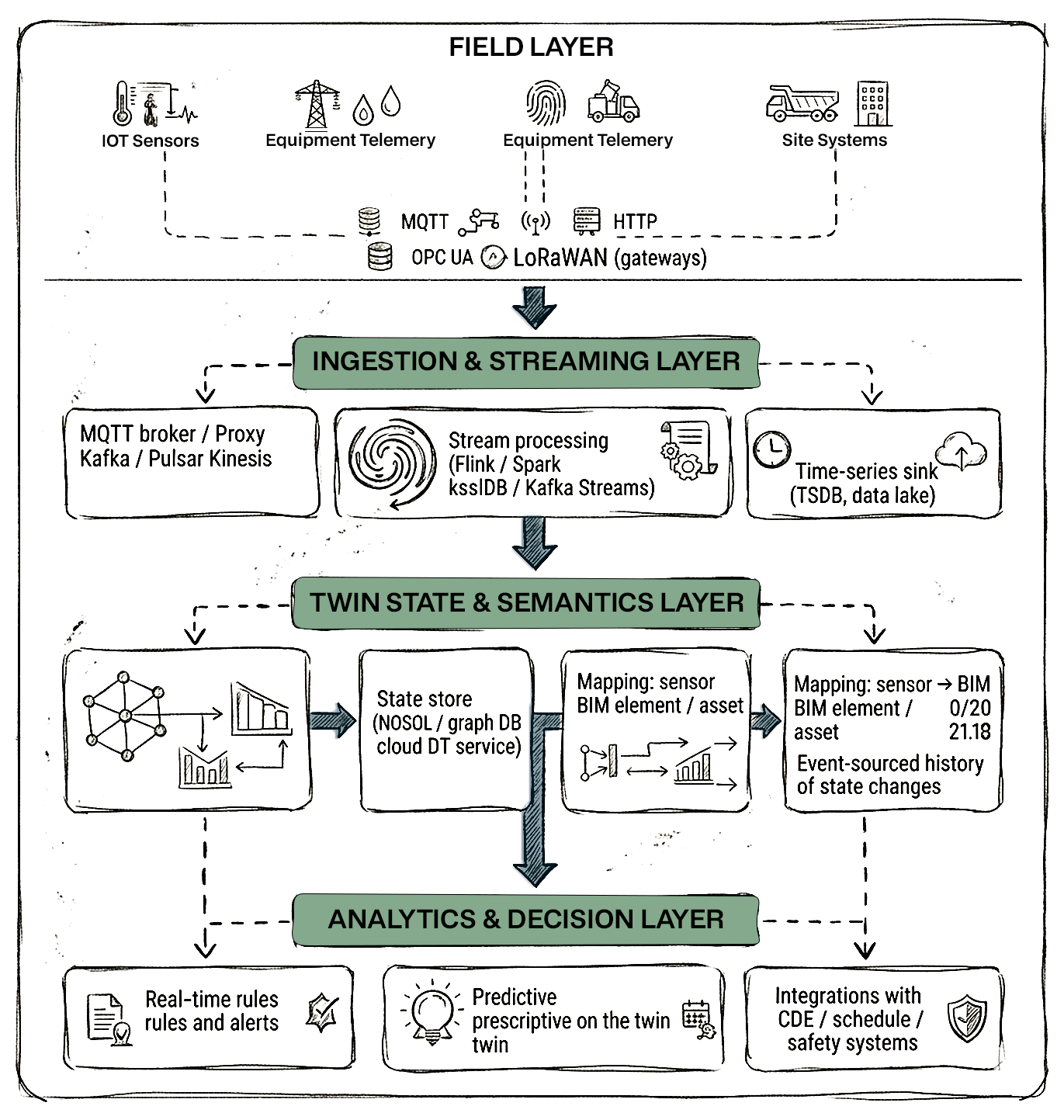
Technologies vary (Kafka vs. Kinesis vs. Zerobus Ingest, Azure Digital Twins vs. custom graph, Lakebase vs. Redis), but the logical responsibilities are consistent across implementations.
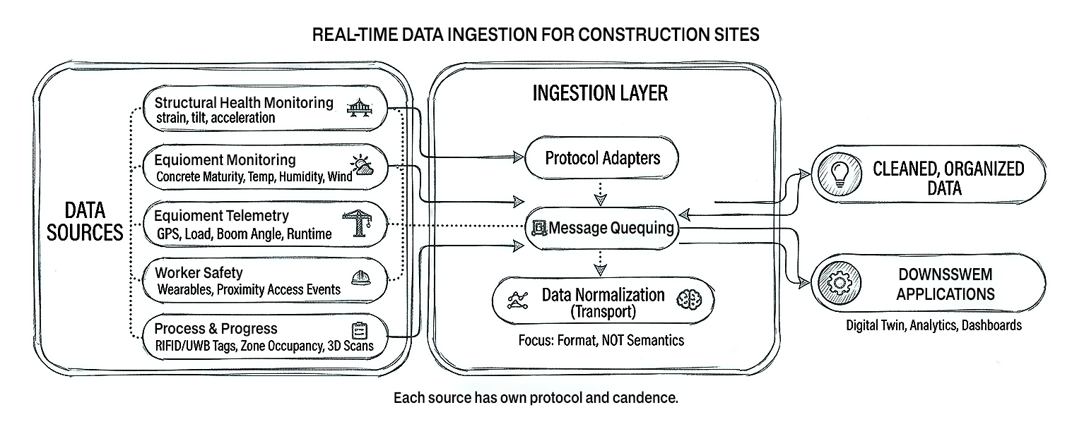
On a construction site, typical real-time data feeds include:
Each source has its own protocol and cadence. A robust ingestion layer normalizes transport, not semantics: it standardises how data is moved and buffered (MQTT, HTTP, OPC UA, custom gateways) without trying to impose business meaning at this stage.
In practice, real-world telemetry is messy. Sensors drift out of calibration over months, are replaced without metadata updates, and experience intermittent data loss due to RF interference, underground works, or power cycles. Gateways may buffer readings during outages and backfill them in bursts once connectivity returns. The ingestion tier must surface these behaviours explicitly: health metrics for each sensor, calibration cycles, and clear flags for backfilled versus live data so downstream logic can treat them differently.
For safety‑critical workflows, delivery and ordering semantics matter as much as throughput. The platform needs to define per‑sensor (or per‑asset) ordering guarantees, decide whether streams are processed under at‑least‑once or effectively‑once semantics, and implement idempotent writes and deduplication so that replays do not generate duplicate alarms. Late‑arriving or out‑of‑order events must be handled with explicit policies: for example, whether a late high‑wind reading should still trigger a stop‑work condition or only adjust historical analytics. These choices sit in the ingestion layer because they govern how “truth” from the field is reconstructed before any domain rules or twin logic run.
There are two primary architectural patterns for getting field data into the analytics platform:
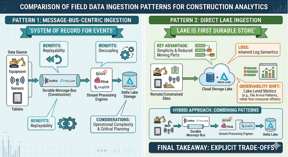
There are two common architectural categories for getting field data into the analytics platform: message‑bus‑centric and direct lake ingestion.
In this model, field gateways publish sensor messages onto a durable message bus (for example, Kafka or Pulsar) using topics that reflect site, zone, asset, or sensor type. The bus becomes the system of record for events, and stream processors (Spark, Flink, ksqlDB, etc.) consume from it to write into the lakehouse and drive downstream logic.
The main advantages are replayability and decoupling. Historic windows can be replayed from the bus into new consumers without touching the source systems, and multiple independent services (twin state updater, anomaly detection, safety alerting) can subscribe to the same topics with their own offsets. On the downside, operating a distributed message bus adds infrastructure and operational complexity: capacity planning, retention policies, partitioning strategy, and monitoring all become part of the critical path.
In a direct‑to‑lake pattern, field agents or lightweight collectors write events straight into the lakehouse (for example, into Delta tables) over managed ingestion services. There is no central message bus; the lake becomes the first durable store. This reduces moving parts and can be attractive on constrained or remote sites where running and maintaining a full message bus cluster is impractical.
The trade‑off is that replay and fan‑out need to be designed differently. You gain simplicity and often lower operational overhead but lose the inherent event log semantics of a dedicated bus. Reprocessing is done from lake storage rather than from an ordered event stream, and observability must come from lake‑level metrics (ingest lag, file arrival patterns, schema evolution) rather than consumer offsets and topic lag.
In practice, many teams adopt a hybrid: a lightweight message broker at the edge for buffering and local replay, with either a central bus or a managed direct‑ingest service upstream. The key is to make the trade‑offs explicit: replayability versus simplicity, degree of decoupling between producers and consumers, and how much operational complexity the team is willing to own for observability and control.
Whether using Kafka topics or Delta tables as the landing zone, a consistent naming convention matters:
iot.raw.environment.siteA.level5.*

iot.raw.structural.bridgePier3.*

iot.raw.equipment.crane1.*

iot.raw.safety.turnstileGate2.*

bim.metadata.*
A Schema Registry enforces consistent structure:
{

  "type": "record",

  "name": "SensorReading",

  "fields": [

    { "name": "sensor_id", "type": "string" },

    { "name": "ts_utc", "type": "long" },

    { "name": "measure_type", "type": "string" },

    { "name": "value", "type": "double" },

    { "name": "unit", "type": "string" },

    { "name": "site_id", "type": "string" },

    { "name": "raw_payload", "type": "string", "default": "" }

  ]

}
The ingestion layer's job is not to understand BIM—it's to reliably land clean, timestamped, schema-validated events into the streaming platform or lakehouse.
Topic and table design also implies a partitioning and retention strategy. For high‑volume telemetry, partitions are often aligned to time (for example, by day) and sometimes site or asset class, so that common access patterns — such as “last 7 days of crane telemetry for Site A” — hit a small, contiguous set of partitions. Retention needs to distinguish between raw event history used for replay or forensic analysis and aggregated views used for day‑to‑day operations; the former may be stored at lower cost tiers with longer retention, the latter in performance‑optimised tables. These choices should be governed centrally, with clear policies on how long different data classes are kept and how they move between storage tiers.
Schema evolution is unavoidable as sites, sensors, and BIM models change. A governed schema registry must support backward‑compatible changes (adding optional fields, new measure types) while detecting and blocking breaking changes that would invalidate downstream consumers. In a real construction project, BIM entities can be re‑modelled across revisions, and IFC GUIDs or internal identifiers may change. Version management becomes critical: every event should be associated not only with a stable twin identifier (IRI) but also, where relevant, with the BIM model version it was derived from, so that historical queries can reconcile telemetry with the correct revision of the design. Without this discipline, mapping drift between the physical assets, the BIM model, and the twin state will quietly erode trust in the system.
Once raw telemetry lands in the bronze layer (Kafka topics or Delta tables), it must be transformed into twin-ready events. This is where BIM semantics enter the pipeline.
A critical step is ensuring that every measurement is labeled with the unique identifier of the entity it represents in the twin model. The Databricks approach uses IRIs (Internationalized Resource Identifiers), a namespaced identifier standard from RDF that uniquely identifies each entity and connects it to telemetry data.
In a construction context, this means mapping:

In the Databricks accelerator, this mapping uses the spark-r2r library, a DSL following the R2RML standard for describing mapping transformations in Spark. The same concept applies regardless of tooling—the mapping from sensor IDs to BIM GUIDs or IRIs must be versioned, traceable, and auditable because wrong mapping leads to dangerous safety decisions.
In live projects, the bigger risk is not a single obvious mis‑mapping but mapping drift over time. Sensors are relocated as temporary works are installed or removed, equipment is repurposed between zones, and BIM models are revised with new GUIDs or re‑modelled assemblies. If these changes are not systematically reflected in the sensor‑to‑IRI mapping, the twin will continue to look “healthy” while readings are silently attached to the wrong physical elements. For safety‑critical use cases ; such as formwork release or crane wind limits ; this can mean alarms triggering on the wrong asset, or worse, not triggering where they should. Treating mapping updates as controlled configuration changes, with approvals, effective‑from timestamps, and full audit history, is therefore as important as calibrating the sensors themselves.
The Databricks approach converts tabular sensor readings into timestamped RDF triples with three components:
The timestamp is modelled explicitly, typically as an additional property (for example, measures:observedAt with an xsd:dateTime literal) or, in some implementations, via quads or named graphs where the fourth element encodes context such as acquisition time or data source. The key point is that every reading carries both what was measured and when it was measured, even though the RDF triple itself remains a three‑component structure.
This triple structure is independent of the source table format, making it a universal representation that works regardless of which sensors, protocols, or data formats are in use across the construction site.
Crucially, adding a timestamp to every triple enables viewing the state of the system at any particular point in time—essential for incident investigation, compliance audits, and time-series analytics on the twin.
The following is illustrative pseudo-code using a Flink/ksqlDB-style syntax to show the enrichment and aggregation pattern. Exact syntax will vary depending on your stream processing framework (Spark Structured Streaming, Flink SQL, ksqlDB, etc.):
-- Enrich sensor readings with BIM asset mapping

CREATE STREAM enriched_sensors AS

SELECT S.ts_utc,

M.twin_iri,

M.zone_id,

S.measure_type,

S.value,

S.unit

FROM sensor_readings S

JOIN sensor_to_asset_map M

ON S.sensor_id = M.sensor_id;

-- PSEUDO-CODE: Calculate concrete maturity index per pour entity

-- Watermark defined on event time to bound lateness

CREATE TABLE concrete_maturity AS

SELECT twin_iri,

HOPPING_WINDOW(ts_utc, INTERVAL '10' MINUTE, INTERVAL '1' HOUR) AS win, AVG(value) AS avg_temp,

COUNT(*) AS samples

FROM enriched_sensors

WHERE measure_type = 'concrete_temp'

GROUP BY twin_iri, win;

-- PSEUDO-CODE: Handle late-arriving events explicitly

-- Events arriving after the watermark threshold are flagged,

-- not silently dropped, so downstream logic can decide treatment

CREATE TABLE concrete_maturity_with_late AS

SELECT twin_iri, win, avg_temp, samples,

CASE

WHEN ts_utc < CURRENT_WATERMARK() THEN 'late'

ELSE 'on-time'

END AS arrival_status

FROM concrete_maturity;
The watermark defines the maximum expected lateness for event-time processing ; in this example, 2 minutes. Events arriving within that window are included in the window computation normally. Events that arrive after the watermark threshold are classified as late and should be handled with an explicit policy: for safety-critical streams such as structural or wind readings, late events may still need to trigger re-evaluation of alerts rather than being silently discarded. For lower-priority analytics streams, they can be written to a separate late-arrival table for asynchronous backfill. The choice of watermark lag is therefore not arbitrary ; it should be calibrated against your sensor transmission cadence, network latency on site, and the safety tolerance of the downstream use case For Databricks-based implementations, this processing runs as Lakeflow Spark Declarative Pipelines that handle large volumes cost-effectively with low latency, outputting silver/gold Delta tables that feed the twin state.
The digital twin is not just an IFC file or Revit model in the cloud. It is a graph of entities with mutable state.
1. Twin Entity Model
At minimum, define:
The twin model can be created using RDF, an open standard for defining knowledge graphs and ontologies. Built-in predicates describe relationships and dependencies between parts of the system, and can be extended for construction-specific semantics. Each entity gets an IRI that uniquely identifies it and connects it to telemetry data in the twin graph.
A graph DB (Neo4j, JanusGraph), a cloud DT service (Azure Digital Twins, AWS IoT TwinMaker), or the Databricks approach with RDF triples in Delta Lake can store this graph.
2. State Store and Event-Sourced Updates
The current state of each twin entity is a materialized view computed from events:
Implementation pattern:
{

  "twin_id": "siteA:structure:column:GUID-1234",

  "ts_utc": 1738790400000,

  "state": {

    "max_strain_24h": 210.5,

    "strain_status": "warning",

    "safety_factor": 1.3

  },

  "cause": "sensor_agg_update"

}
This separation of concerns is crucial: stream processors are the brains; the twin store is the memory.
3. Operational Serving: Bridging Analytics and Applications
A common challenge with digital twins is serving twin state at low latency for operational applications while retaining full history for analytics. The Databricks architecture addresses this with a Reverse ETL pattern using Lakebase Synced Tables:
This means a construction site supervisor's mobile app can fetch the latest crane status or concrete maturity estimate with Postgres-speed queries, while the data science team runs complex time-series models against months of history in Delta Lake—both from the same source of truth.

Analytics is layered on the twin, not on raw tags. That's where BIM semantics shine.
1. Real-Time Monitoring & Alerts
Rules are now expressed in terms of twin entities:
These rules are much easier to manage when the twin graph already links:
Complex rules can run in stream-processing engines (Flink CEP, Kafka Streams, ksqlDB), rule engines subscribing to twin.state.*, or ML models (anomaly detection, risk scoring) invoked from these pipelines.
2. Querying the Twin with SPARQL
For implementations using the RDF-based twin model, the powerful SPARQL query language enables ad hoc analysis and fault propagation queries. This is an open standard for knowledge graph querying—in contrast to proprietary query languages offered by some twin platforms.
Example construction query: "Which structural elements in Zone L5-East share a dependency chain with the sensor showing anomalous strain readings?" — a graph traversal that's natural in SPARQL but complex in relational SQL.
3. Predictive & Prescriptive Models
Examples relevant to construction:
After initial deployment, more advanced applications can be layered on:
Prescriptive actions flow back into operational systems:
The twin offers a shared context for these models: they use the same IDs and relationships as planners, engineers, and supervisors.
Predictive models in construction face a fundamental bootstrapping problem: the volume and quality of labelled historical data required to train a reliable model simply does not exist at the start of a project. A concrete curing model needs dozens of comparable pour records across varied mix designs, ambient conditions, and insulation configurations before its predictions are trustworthy.
An equipment failure model needs run-to-failure events : which are rare by design in well-maintained fleets. This cold-start problem means that for the first weeks or months of a project, ML-based predictions should be treated as indicative rather than actionable, and rule-based thresholds and physics-based models (such as the Nurse-Saul maturity equation for curing) should carry the primary decision weight.
Alongside cold-start, teams must also address data sufficiency thresholds explicitly: define, for each model, the minimum number of samples, the minimum coverage of conditions, and the minimum sensor uptime required before the model is promoted to production. Deploying a model before these thresholds are met : particularly in safety-critical workflows : introduces risk that is difficult to detect because the model will produce confident-looking outputs even on insufficient evidence.
The cold-start challenge has a practical mitigation: construction projects within the same programme, portfolio, or asset class generate structurally similar data. Concrete poured with the same mix in similar ambient conditions, cranes of the same type under comparable load cycles, and safety zones with equivalent activity profiles all produce signals that can inform models beyond a single project.
Organisations that architect their twin pipelines with cross-project learning in mind can seed a new project's models with priors derived from historical data across the portfolio, significantly compressing the cold-start period.
This requires deliberate data normalisation: IRI-based entity identifiers need to be portable across projects (or mapped to shared canonical identifiers), sensor telemetry schemas must be consistent, and the mapping between physical conditions and model features must be documented and transferable.
In practice, this points toward a centralised feature store or a shared gold-layer dataset that retains model-ready features from closed projects. Over time, this institutional memory becomes a competitive advantage: each new project starts with a richer prior, and the organisation's models improve faster than those of teams treating each project as a data island.
Analytics models running on twin data do not stay accurate indefinitely. Sensor drift, site configuration changes, and seasonal variation in construction activity all cause model inputs to shift over time, degrading prediction quality without obvious failure. Model monitoring should be a first-class operational concern: track input feature distributions against a baseline, monitor prediction confidence and alert volume trends, and flag when a model's behaviour has deviated beyond a defined threshold.
In a construction context, this is particularly relevant for models that influence scheduling or formwork release decisions, where a quietly degrading model can introduce systematic bias into critical path estimates.
Safety-critical systems face a specific failure mode that purely technical metrics miss: alert fatigue. If a crane wind-limit model or zone-breach detector fires too frequently on non-actionable conditions, operators begin to ignore it ; and the system's safety value erodes regardless of its technical accuracy. False positive management must therefore be built into the operating model from the start.
This means logging every alert, tracking acknowledgement and override rates, and reviewing high-frequency alerts in a structured cadence. Where overrides are common, the root cause should be investigated: the threshold may need tuning, the sensor may be drifting, or the rule logic may not account for a legitimate site condition. Override rates are also a governance signal ;a high rate on a safety-relevant alert should trigger a formal review rather than informal workarounds.
In safety-critical workflows, opaque decision logic is not acceptable. If the twin recommends holding a formwork stripping activity or issues a stop-work alert, the responsible engineer must be able to understand and verify the basis for that recommendation ; not simply trust a model score. This requires building explainability into the analytics layer: surface the specific sensor readings, thresholds, and rules that contributed to a recommendation alongside the recommendation itself.
For ML-based components, techniques such as feature contribution scoring (for example, SHAP values) can make individual predictions interpretable, but the output should always be presented in terms of physical conditions ; "estimated concrete strength is currently 68% of design threshold, based on slab temperature readings from the last 4 hours" ;rather than raw model outputs.
Every decision the twin influences should be logged with a full audit trail: what data was available, what logic fired, and what recommendation was issued. This record is essential not just for operational review but for incident investigation and regulatory compliance.
Building a construction digital twin is fundamentally a data engineering problem before it is anything else. The architecture described across these sections — from MQTT-based sensor ingestion and Zerobus Ingest to RDF-based twin state modeling and Lakebase-powered operational serving — forms the technical foundation that separates a passive 3D model from a live, decision-ready system.
The key principles to carry forward:
With this pipeline in place, the twin is ready to do what it was actually built for: change decisions on the ground, not just display data on screens.