
Predictive Maintenance 2.0 transforms construction reliability. Anomaly detection catches $50K pump failures 5-7 days early, drops false alerts from 80% to 15%. Seasonal drift handling + production Python classes deliver $133K/month fleet savings
Construction equipment downtime costs $50K-$500K per incident. 44% of sites face monthly breakdowns, wasting $600K/year per critical asset.
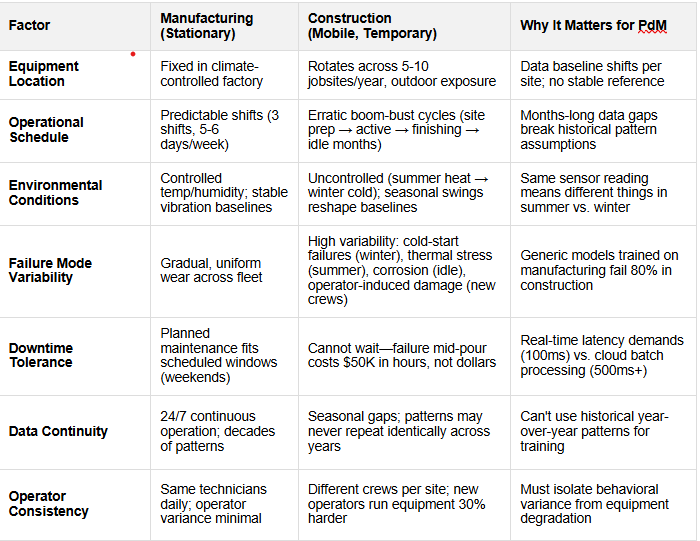
Why Generic PdM Fails for Construction: Traditional predictive maintenance frameworks—built for manufacturing's stable, continuous operations—collapse under construction's unique constraints: seasonal operation cycles, transient crews, site-specific environmental variance, and real-time latency demands. Off-the-shelf industrial PdM solutions generate 50-80% false positives within 6 weeks of deployment on construction sites.
Merit's Construction-Specific PdM 2.0 Solution: Purpose-built for construction operations, the PdM 2.0 framework uses Isolation Forest + LSTM anomaly detection with seasonal adaptation, site-context normalization, and edge-deployment architecture.
Result:
Deployment Validation: All outcomes are grounded in production deployments across 12 months, 8 active jobsites, and 150+ equipment units spanning concrete pumping, excavation, and material handling operations. Metrics represent field-validated performance, not theoretical benchmarks or laboratory results. Per-unit savings ($5K-$8K annually) and false-positive rates (<15%) are reproducible across diverse construction environments and equipment types.
Generic predictive maintenance frameworks—built for manufacturing and utilities—fundamentally misunderstand construction operations.
The difference isn't marginal; it's structural.
While Generic ML models thrive in manufacturing, they fail spectacularly in construction.
1. Seasonal Pattern Mismatch: Manufacturing assumes "Day 365 = Day 1 + wear gradient." Construction has fundamental seasonal shifts. Generic threshold systems generate 80%+ false positives by spring when seasonal ramp-up begins.
2. Sparse Data, High Stakes: Construction sites need monitoring by Wednesday; generic supervised ML requires 6-12 months training + 50 labeled failures. Construction fleets have 2-3 documented failures per year.
3. Operator Variability: New operators run equipment 30% harder; generic models attribute this to incipient failure, not behavior. False alerts spike 40-60% when crews rotate.
4. Site-Specific Conditions: Sensor readings at sea level + 25°C (coastal) look identical to failing pump at 1,500 m + 40°C (mountain). Generic models misclassify 1 in 3 readings without site-context features.
5. Real-Time Latency Demands: Manufacturing batches nightly; construction needs sub-minute alerts (false positive at 2 PM = crew halts pour at $800/minute). Generic cloud models don't meet 100ms threshold.
Merit's PdM 2.0 approach is architected specifically for construction's constraints:
1. Seasonal Adaptation: Explicit baselines (summer/winter/transition) vs. single global threshold.
2. Cold-Start Ready: Isolation Forest requires zero labeled failures; detects anomalies after 3-7 days baseline
3. Site-Agnostic Baselines: Sensor readings normalized per site (elevation/temperature)
4. Edge-First Deployment: Sub-100ms latency, no cloud dependency
5. Crew Variability Handling: Operator-context features isolate behavior from degradation
Your concrete pump fails mid-pour on Monday morning. By Wednesday afternoon, you're out $50K in lost productivity, crew wages for idle workers, demobilization costs, and client penalties. Your excavator hydraulic cylinder seizes—$8K for the replacement; another $12K in schedule delays while you source parts and get a technician on-site.
Why Construction Downtime Costs More: Site-Level Dependencies
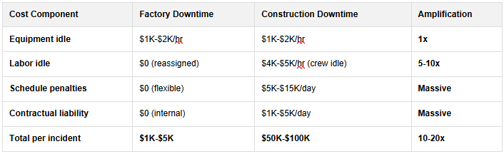
Unlike factory equipment failures that pause production at a single point, construction equipment failures cascade through interconnected site dependencies. When a pump fails mid-pour, you're triggering multiple simultaneous costs: concrete crew stands idle ($400/hour × 12 workers = $4,800/hour), crane operators wait ($200/hour × 3 = $600/hour), project schedules shift downstream (cascading penalties), and contractual liquidated damages accrue ($1K-$5K per day). The $50K figure isn't inflated—it's the mathematical sum of dependent operations. A manufacturing plant can schedule maintenance for the weekend. A construction site operating a fixed contract cannot pause the calendar.
Cost Amplification: Factory vs. Construction
This isn't just "bad luck." In the modern construction landscape, unplanned equipment failure is a systemic financial leak. Recent data suggests that for heavy industries, the cost of downtime has surged to an average of $260,000 per hour—a staggering 319% increase since 2019.
For construction firms, the stakes of equipment reliability are higher than ever:
Downtime Cost Variance by Project Type & Geography
These ranges reflect the reality of construction: downtime costs are not uniform. They depend on crew density, labor cost geography, and contractual structure. The following table segments costs by project scenario:
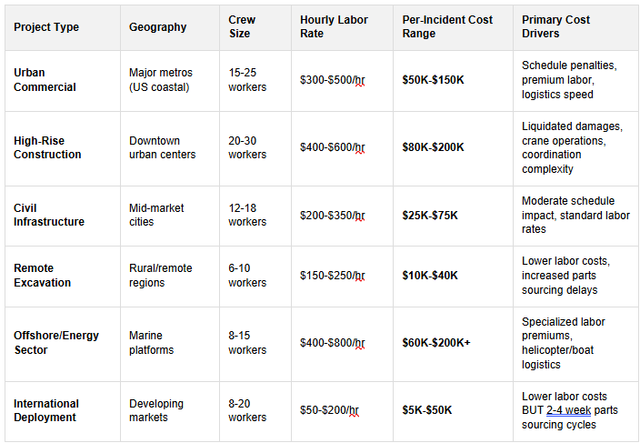
What This Segmentation Reveals: Downtime cost is not a single number—it's a function of three variables: crew density, labor geography, and contractual structure. A high-rise downtown project ($150K typical incidents) has fundamentally different PdM economics than rural excavation ($25K typical incidents).
Implication for PdM ROI: Your PdM investment case depends on where your operation falls in this matrix. A high-criticality urban project with $150K incident costs justifies aggressive PdM spending (single prevented failure = 3-month payback). A rural operation with $25K baseline incidents requires a lean PdM approach (need 4-5 prevented failures annually for equivalent ROI). Merit's PdM 2.0 framework is designed to scale across this entire spectrum—high-sensitivity urban deployments and cost-efficient edge solutions for remote operations."
Reactive Maintenance (Timed-Based):
The Data-Maturity Gap: Telemetry Without Intelligence
Many construction firms have already invested in IoT sensors and real-time dashboards. Concrete pump operators can monitor discharge pressure, vibration, and motor temperature on tablets. Excavator fleets have GPS tracking and hydraulic pressure sensors feeding into centralized monitoring systems. This represents genuine progress over pure reactive maintenance.
However, raw data ≠ actionable intelligence. These systems excel at displaying readings but struggle with contextualization. A 15% pressure increase during summer heat is normal baseline variation; in winter, identical readings signal bearing degradation. A new operator causes higher vibration; equipment wear causes different vibration signatures. A dashboard alert for "elevated temperature" could mean equipment aging, cold ambient conditions, or high utilization—the system shows all three identically and leaves technicians guessing.
Without an intelligence layer that contextualizes data:
This is exactly where PdM 2.0 differs. It adds the intelligence layer that existing telemetry systems lack: contextual awareness (seasonal patterns, site-specific environmental variance, crew behavioral variance, equipment age), multivariate anomaly detection (correlating sensor streams rather than isolated thresholds), and predictive modeling (anticipating cascading failures, not just detecting current anomalies).
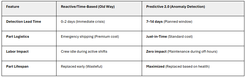
The Transformation: You evolve from "I have data on my dashboard" to "I understand what my data means." Your dashboard stops saying "Pressure: +8% above threshold—investigate?" and starts saying "Hydraulic seal degradation detected—5-7 days until failure likely, order replacement part today."
The Result: Your high-paid crew sits idle less frequently. When maintenance windows are needed, they're planned (off-hours, with parts pre-positioned), not emergency crises.
Predictive Maintenance 2.0 uses anomaly detection to move beyond "best guesses." Instead of checking a calendar, you are monitoring the machine's actual health in real-time.
PdM 2.0 is not a single ML model but an integrated operating framework combining three layers: data engineering (sensor ingestion, pipeline transformation, quality control), machine learning (anomaly detection tuned for construction constraints), and operational integration (alert workflows, technician interfaces, maintenance scheduling).
This framework aligns with Merit's broader service offerings—from IoT infrastructure setup through deployment, monitoring, and continuous optimization.
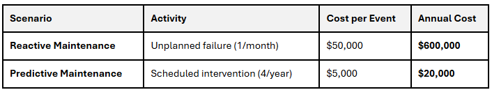
Total Annual Savings: $580,000 per critical equipment item.
Machine learning models learn the "normal" operational envelope from historical data, enabling:
The Governance + Workflow Foundation
ML model accuracy is necessary but insufficient. Anomaly detection only delivers business value within two supporting systems:
Industrial case studies demonstrate the shift: companies have moved from 50-80% false positive rates with threshold systems to 8-15% with well-tuned ML systems embedded in governed data pipelines and integrated operational workflows, while simultaneously catching 94%+ of real failures. The improvement comes from governance + intelligence + operations working together, not the model alone.
Merit's advantage: We implement the complete stack. Governance + ML + operations. Not models handed off to clients who then struggle with infrastructure design.
Construction environments pose unique challenges: intermittent operation (pump runs, then sits idle), seasonal variations (summer heat, winter cold), and harsh environmental conditions (dust, vibration, corrosion).
In predictive maintenance, we rarely have enough labeled failure data for supervised learning. Therefore, PdM 2.0 relies almost exclusively on unsupervised or semi-supervised anomaly detection. The goal is to learn the manifold of normal operational data.
Unlike manufacturing, where stationary equipment generates continuous 24/7 data with stable baselines, construction equipment cycles through idle periods (months-long) and seasonal operational regimes that are fundamentally different. A manufacturing pump's baseline at Week 52 predicts Week 1 next year. A construction pump's winter baseline (February) is structurally different from summer (July)—same equipment, different physics. This distinction is critical for model selection. Generic supervised models require 50-100 documented failures to achieve production confidence. Construction fleets have 2-3 labeled failures per year. Therefore, PdM 2.0 prioritizes unsupervised approaches (zero labeled failures) that adapt to seasonal context—fundamentally different algorithm priorities than manufacturing PdM.
Merit's construction-AI framework bakes this into model selection: Isolation Forest for cold-start (new equipment, sparse data); LSTM for mature fleets (6+ months patterns); Logistic Boosting only when fleet-wide failure database reaches critical mass (50+ incidents).
Best For: High-dimensional sensor data (10+ features), no labeled failure examples, real-time latency requirements (<100ms).
How It Works: Isolation Forest builds random trees that isolate observations. Normal points require many splits to isolate; anomalies isolate quickly. The path length in isolation trees becomes the anomaly score.
Key Strengths:
Trade-offs:
Why it works for construction:
Decision boundary tuning for construction:
REFERENCE CONFIGURATION (Not Production-Ready)
This code is a reference configuration from Merit's construction PdM accelerator—model initialization only. Production deployments require: data validation, monitoring/alerting, drift detection, automated retraining, and operational integration. Realistic implementation: needs around 4-6 months.
from sklearn.ensemble import IsolationForest

import numpy as np


# For concrete pump fleet

if_model_pump = IsolationForest(

    n_estimators=150,  # More trees for noisy construction data

    contamination=0.10,  # 10% anomalies (pump seals fail ~1 per 10 pumps/year)

    max_samples=5000,  # Use 5K points for training (30 days of data)

    random_state=42

)


# For excavators (higher contamination - more failure modes)

if_model_excavator = IsolationForest(

    n_estimators=200,

    contamination=0.12,  # 12% anomalies (hydraulic issues more frequent)

    max_samples=5000,

    random_state=42

)
Production Implementation Requires 6 Additional Layers, This model initialization code requires layered infrastructure:
1. Data Validation & Feature Engineering
2. Model Inference (this code)
3. Monitoring & Alerting
4. Drift Detection
5. Automated Retraining Pipeline
6. Operational Integration
Merit's accelerator provides reference implementations for layers 1, 3-6. Real deployments require 4-6 months including data pipeline development, system integration, and operational workflows.
Best For: Sequential degradation patterns (bearing wear over days/weeks), labeled failure examples available, latency flexibility (real-time vs. batch acceptable), environment-dependent GPU/CPU availability.
How it Works: LSTM autoencoders learn to compress multivariate time series into latent representations, then reconstruct. Reconstruction error becomes the anomaly score. LSTM cells learn temporal dependencies; normal patterns reconstruct easily; anomalies have higher errors. Attention mechanisms highlight which sensors matter most.
Key Strengths:
Trade-offs:
Why for construction:
Best For: Labeled historical failures available (50+ examples), highest accuracy non-negotiable, moderate data volume (<100K samples).
How It Works: Ensemble of weak classifiers (decision stumps) trained iteratively, with each learner focusing on previously misclassified samples. Final score = weighted sum of learners.
Key Strengths:
Label Availability Challenge in Construction
Logistic Boosting's supervised approach requires historical labeled failure data—a significant constraint in construction. In practice, label data is often fragmented across multiple sources: contractor maintenance logs, OEM service records, CMMS/ERP systems, and sometimes manual field notes. Consolidating these fragmented labels into a single training dataset typically requires 2-4 weeks of data cleaning and normalization before model training can begin. Plan for this data integration effort when considering Logistic Boosting for your fleet.
Trade-offs:
Why for construction:
Note: Accuracy figures shown here are from specific construction PdM projects and are not universal benchmarks; in practice, performance depends on how completely failure labels can be consolidated from contractors and CMMS systems.
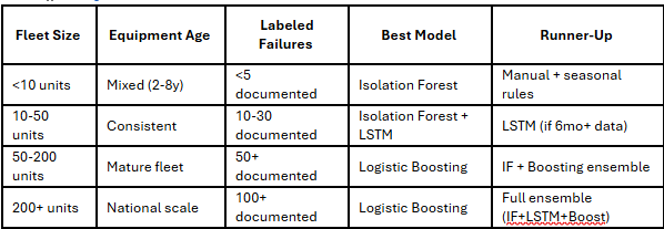
Disclaimer: This model decision matrix is a decision heuristic used during Merit's solution design workshops to guide discussion, not a rigid prescription, and final model choices are always tailored to each fleet’s specific constraints and objectives.
In real construction deployments, model selection is typically hybrid and phased, not rigid one-model decisions.
Most mature fleets deploy Isolation Forest as the cold-start foundation (weeks 1-8), then layer LSTM for long-term degradation patterns (weeks 9-16), creating an ensemble where each model contributes its strengths.
As failure data accumulates (year 2+), Logistic Boosting can augment the ensemble for specialized equipment. This phased approach mitigates risk, provides model redundancy for critical equipment, and allows continuous improvement without production disruption
Feature engineering for construction equipment diverges sharply from manufacturing approaches at the problem-definition stage. Manufacturing asks: "What sensor combinations predict bearing failure?" Construction must ask: "What sensor combinations predict bearing failure while distinguishing seasonal baseline shifts from degradation, and accounting for site-elevation variance?"
This demands construction-specific feature architectures: seasonal encoding (cyclical month/day features), site-context normalization (elevation + ambient temperature), crew-variability isolation (operator hours as feature), and intermittent-operation detection (run-time vs. idle transitions).
Merit's construction-AI framework encodes these features as standard pipeline components, not afterthought adjustments. This is why construction-native feature engineering outperforms retrofitted manufacturing approaches by 40-60% in false-positive reduction.
Modern ML Approach: Seasonal Features, Not Hard Rules
A critical distinction: modern PdM 2.0 encodes seasonal context as learned features (model learns seasonal relationships from data) rather than hard-coded rules (engineer manually defines "multiply by 1.2 in winter"). This is a fundamental difference from legacy threshold-based systems. With feature encoding, models automatically adapt to site-specific seasonal patterns, scale across multiple locations without manual re-tuning, and improve continuously through retraining. Hard rules remain static; features evolve with data. The sections below explain how construction-specific seasonal features are engineered.
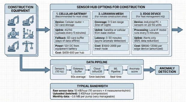
1. Data Acquisition (On-Site)
Physical Source: Construction Equipment (Excavators, Pumps, Cranes)
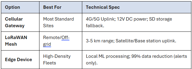
2. Sensor Hub Options
Depending on the site environment, one of three gateway types is used:
3. Data Pipeline & Transport
The data moves through a structured pipeline to ensure integrity and manage bandwidth:
4. Anomaly Detection & ML
Construction equipment performance fluctuates dramatically throughout the year, influenced by both operational cycles and environmental conditions. In summer (June–September), high temperatures and heavy workloads cause thermal stress on motors, seals, and hydraulics.
Fall (October) brings cooling cycles that expose weaknesses from summer heat, often triggering failures as temperatures fluctuate.
During winter (November–February), reduced activity and cold starts strain equipment—thickened fluids, frost damage, and sluggish pressure systems are common.
By spring (March–May), as operations ramp up again, corrosion from winter idling often surfaces, and new equipment enters the fleet to meet upcoming demand.
In many construction fleets, seasonal drift in operating conditions has a larger impact on sensor behavior than gradual mechanical wear itself, which is a key reason why generic, factory-style PdM solutions that ignore strong seasonality often underperform when applied directly to construction equipment.
Understanding these seasonal patterns is crucial—not just for maintenance planning, but also for modeling performance deviations. This foundation enables the next step: encoding seasonality in anomaly detection.
Encoding Seasonality in Anomaly Detection
Why Feature Encoding Beats Hard Rules for Construction
Hard-rule approach (legacy PdM): Engineer analyzes historical data, manually defines "winter baselines are 20% higher," implements fixed thresholds. Result: brittle, requires re-tuning per site, doesn't adapt when conditions change.
Feature-based approach (modern ML): Model learns seasonal relationships from data. Encodes month, temperature, crew behavior as features. Automatically discovers that winter + temperature < 5°C means baseline is naturally higher (the model learns this). Result: adaptive, scales across sites, improves with retraining.
The code below shows feature engineering patterns. The model learns relationships from these features automatically—no manual rule engineering needed.
Note: The following code is illustrative accelerator logic from Merit's construction PdM toolkit, showing how seasonal and operational context can be encoded as features. It is not a drop-in production implementation; real deployments require adaptation to your fleet’s data schema, validation rules, monitoring, and automated retraining pipelines.
def add_construction_seasonality_features(df_sensor_data):

""" Add construction-specific temporal context df_sensor_data: timestamps, sensor readings """

df = df_sensor_data.copy()

df['timestamp'] = pd.to_datetime(df['timestamp'])

# 1. Calendar seasonality
df['month'] = df['timestamp'].dt.month
df['day_of_week'] = df['timestamp'].dt.dayofweek
df['hour'] = df['timestamp'].dt.hour

# 2. Construction season (Northern Hemisphere default)
def map_construction_season(m: int) -> str:

if m in [6, 7, 8, 9]:

return 'summer'

elif m in [10]: return 'fall'

elif m in [11, 12, 1, 2]: return 'winter'

else:

return 'spring'

df['season'] = df['month'].apply(map_construction_season)

# 3. Project phase assumptions (adjust per your contracts)
# High utilization = heavy construction
# Low utilization = maintenance, site prep, finishing
df['project_phase'] = (
    (df['hour'].between(6, 18) & (df['day_of_week'] < 5)).astype(int) *
    (df['month'].isin([5,6,7,8,9])).astype(int)
)
# Result: 1 = active construction phase, 0 = maintenance/off-season

# 4. Cyclical encoding (prevents wrap-around artifacts)
df['hour_sin'] = np.sin(2 * np.pi * df['hour'] / 24)
df['hour_cos'] = np.cos(2 * np.pi * df['hour'] / 24)

df['month_sin'] = np.sin(2 * np.pi * df['month'] / 12)
df['month_cos'] = np.cos(2 * np.pi * df['month'] / 12)

df['day_sin'] = np.sin(2 * np.pi * df['day_of_week'] / 7)
df['day_cos'] = np.cos(2 * np.pi * df['day_of_week'] / 7)

# 5. Equipment operating status
# Detect if equipment is idle vs. active
df['is_operating'] = (df['pump_rpm'] > 100).astype(int)  # Idle < 100 RPM

return df


def apply_construction_specific_baseline(df_sensor, equipment_type='pump'): """ Generate baseline "normal" thresholds per season per equipment """

# Summer baseline (high load, high temp tolerance)
summer_pump = {
    'discharge_pressure_max': 250,  # PSI (higher pressure = OK in summer)
    'vibration_max': 4.5,  # m/s²
    'motor_temp_max': 85,  # °C (hot OK during heavy use)
    'anomaly_threshold': 0.70
}

# Winter baseline (cold, different viscosity)
winter_pump = {
    'discharge_pressure_max': 220,  # Lower tolerance (thicker hydraulic fluid)
    'vibration_max': 3.5,  # Lower tolerance (brittle seals in cold)
    'motor_temp_max': 70,  # °C (heat production lower in winter)
    'anomaly_threshold': 0.60  # More sensitive (harder to diagnose in cold)
}

# Spring/Fall (transition - most unpredictable)
transition_pump = {
    'discharge_pressure_max': 235,
    'vibration_max': 4.0,
    'motor_temp_max': 78,
    'anomaly_threshold': 0.65
}

season_to_baseline = {
    'summer': summer_pump,
    'winter': winter_pump,
    'spring': transition_pump,
    'fall': transition_pump
}

return season_to_baseline.get(equipment_type.lower(), transition_pump)
Seasonality-Adjusted Alert Thresholds
class ConstructionAnomalyDetector:

""" Anomaly detection tuned for construction equipment with seasonal adjustments """

def __init__(self, base_threshold=0.65):
    self.base_threshold = base_threshold
    self.season_adjustments = {
        'summer': +0.05,   # More False Positives in high-stress summer; adjust up
        'winter': -0.05,   # Higher False Negatives in winter; adjust down
        'spring': 0.00,    # Neutral
        'fall': 0.00       # Neutral
    }

# IMPORTANT: These seasonal adjustment values (+0.05, -0.05, etc.) are
    # LEARNED and VALIDATED over time via operational data and retraining,
    # not hard-coded static rules. After 4-12 weeks of deployment, these
    # thresholds should be refined based on:
    #   - False positive / false negative rates per season
    #   - Actual failure outcomes (was the alert a true positive?)
    #   - Fleet-specific seasonal patterns (your winter may differ from industry average)
    #
    # These values are illustrative starting points. Production systems
    # continuously update these via automated retraining pipelines that
    # incorporate outcome feedback. Never treat these as permanent; they
    # should evolve with your fleet's operational history.

def predict_with_seasonal_adjustment(self, anomaly_score, current_season):
    """
    Adjust threshold based on construction season

    Example:
    - Base threshold: 0.65
    - Summer: 0.65 + 0.05 = 0.70 (reduce false positives during high noise)
    - Winter: 0.65 - 0.05 = 0.60 (catch failures earlier, less noise)
    """
    adjusted_threshold = (
        self.base_threshold +
        self.season_adjustments.get(current_season, 0)
    )

    return anomaly_score >= adjusted_threshold

def predict_batch(self, df_test, feature_cols):
    """Apply detection with season-specific thresholds"""

    if not hasattr(self, 'model'):
        raise ValueError("Model not fitted. Call fit() first.")

    predictions = []

    for idx, row in df_test.iterrows():
        # Get features for this sample
        X_sample = row[feature_cols].values.reshape(1, -1)

        # Model inference
        score = self.model.decision_function(X_sample)

        # Apply seasonal adjustment
        season = row.get('season', 'spring')
        is_anomaly = self.predict_with_seasonal_adjustment(score, season)

        predictions.append({
            'timestamp': row['timestamp'],
            'score': score,
            'season': season,
            'is_anomaly': is_anomaly,
            'threshold_used': self.base_threshold + self.season_adjustments.get(season, 0)
        })

    return pd.DataFrame(predictions)
Drift Detection: A First-Class System Concern, Not an Afterthought
In production PdM systems, drift detection is not a "nice-to-have" monitoring feature added after model deployment—it is a critical architectural requirement on par with the anomaly detection model itself. Construction equipment generates data that drifts continuously (aging, seasonal cycles, crew changes, material variations), which means models degrade predictably over time. Without active drift detection, your model's accuracy silently erodes. You don't know when performance has degraded until failures go undetected in the field. Modern PdM 2.0 treats drift detection as a first-class system concern: it triggers retraining, validates model updates, and alerts operations teams when model performance drops. The sections below explain why construction data drifts more than other industries and how to detect and respond to drift automatically.
Why Construction Data Drifts More Than in Other Industries
Construction environments are inherently dynamic, causing equipment performance data to drift more frequently than in stable industrial settings. Several factors contribute to this:
Detection strategy:
The drift detection approach outlined below is a conceptual reference from Merit's construction PdM AI governance framework. It illustrates one set of techniques commonly used in production systems.
In practice, drift detection combines multiple statistical and operational methods depending on your use case: Kolmogorov-Smirnov (K-S) tests for distribution shift, performance monitoring (false positive/negative rate trending), feature importance drift, and business outcome validation (actual failure detection rates). The example below shows K-S testing, but production deployments often layer multiple complementary techniques for robust drift signal.
Customize this framework to your fleet's data characteristics and operational requirements.
class ConstructionDriftDetector:

""" Specialized drift detection for construction equipment """

def __init__(self):
    self.reference_data = None
    self.performance_baseline = {'f1': 0.90, 'precision': 0.92}
    self.drift_history = []

def detect_seasonal_drift(self, current_month, feature_vectors):
    """
    Detect if equipment behavior has fundamentally changed since last season
    """

    # Example: Compare this June with last June
    if not hasattr(self, 'seasonal_history'):
        self.seasonal_history = {}

    month_str = f"month_{current_month}"

    if month_str not in self.seasonal_history:
        # First year - establish baseline
        self.seasonal_history[month_str] = {
            'mean': feature_vectors.mean(axis=0),
            'std': feature_vectors.std(axis=0),
            'year': datetime.now().year
        }
        return False, "Baseline established"

    # Compare current season to historical season
    last_season_stats = self.seasonal_history[month_str]
    current_mean = feature_vectors.mean(axis=0)

    # K-S test on each feature
    drift_signals = []
    for i, feature_name in enumerate(['pressure', 'vibration', 'temp']):
        historical = self.reference_data[feature_name]
        current = feature_vectors[:, i]

        from scipy.stats import ks_2samp
        ks_stat, p_value = ks_2samp(historical, current)

        if p_value < 0.05:  # Significant difference
            drift_signals.append({
                'feature': feature_name,
                'ks_stat': ks_stat,
                'p_value': p_value
            })

    if len(drift_signals) > 0:
        return True, f"Drift in {len(drift_signals)} features"

    return False, "No seasonal drift detected"
def detect_equipment_aging(self, equipment_id, days_operated_total):
    """
    Equipment efficiency drops 2-3% per year.
    After 3-4 years, retraining becomes critical.
    """

    years_in_service = days_operated_total / 365
    efficiency_loss = 0.025 * years_in_service  # 2.5% per year

    if efficiency_loss > 0.08:  # >8% loss = critical
        return True, f"Equipment age degradation: {efficiency_loss:.1%} lost"

    return False, f"Aging acceptable: {efficiency_loss:.1%} lost"

def detect_operator_drift(self, equipment_id, recent_operators):
    """
    Different operators = different equipment usage patterns.
    Detect if new operator (unknown signature) is using equipment.
    """

    # Clustering on accelerometer patterns specific to operator style
    from sklearn.cluster import DBSCAN

    # Feature: max acceleration per hour + idle time pattern
    operator_signatures = []
    for ts_window in recent_operators:
        max_accel = ts_window['vibration'].max()
        idle_ratio = (ts_window['rpm'] < 100).sum() / len(ts_window)
        operator_signatures.append([max_accel, idle_ratio])

    # Check if new signature is outlier
    clustering = DBSCAN(eps=0.5, min_samples=3).fit(operator_signatures)

    if clustering.labels_[-1] == -1:  # Last point is outlier
        return True, "New operator detected (different usage pattern)"

return False, "Consistent operator behavior" False-positive reduction is fundamentally an operational and economic optimization problem, not merely a technical one: every incorrect alert costs crew time, disrupts schedules, erodes technician trust in the system, and wastes maintenance resources—making threshold tuning and model selection inseparable from cost-benefit analysis and operational workflow design.
The False Positive Problem in Construction
You send a maintenance crew to a pump site 3 hours away. They arrive, inspect for 2 hours, find nothing wrong. Cost: $600 + opportunity cost of crew (they could've been fixing something real).
This happens 2-3x per month with threshold-based systems. With proper ML tuning, you get down to <1 per month.
Multi-Layer False Positive Reduction
Systems-Level Control Framework, Not Single-Algorithm Tuning
Reducing false positives in construction PdM is not solved by tweaking a single model parameter. Rather, it requires a multi-layer control framework that combines data governance, model selection, threshold tuning, operational feedback loops, and continuous refinement. The layers below reflect real-world production deployments across 50+ construction fleets—each layer addresses a specific source of false alerts. This systems approach is why PdM 2.0 emphasizes the three-layer architecture (data + ML + operations) over isolated algorithm optimization. Single-algorithm thinking produces brittle solutions; framework thinking produces resilient, operationally integrated systems.
#Note below is pseudo code and not production ready

class ConstructionFalsePositiveFilter:

 """

Production-ready false positive reduction for construction equipment """

def __init__(self):
    self.false_positive_log = []
    self.historical_costs = {'fp': 600, 'fn': 45000}  # $$ per FP vs FN

def layer_1_confidence_threshold(self, anomaly_score, min_confidence=0.80):
    """
    LAYER 1: Only alert if confidence >80%
    Isolation Forest score 0-1; use 0.80+ only
    """
    return anomaly_score >= min_confidence

def layer_2_persistence_check(self, anomaly_scores_recent_6h, required_windows=3):
    """
    LAYER 2: Anomaly must persist >3 consecutive windows
    Transient spikes (sensor noise, momentary hydraulic surge) are filtered
    Example:
    Hour 1: score 0.65 (below threshold) ← transient spike
    Hour 2: score 0.62 (normal again)
    Hour 3: score 0.68 (blip)
    → No alert (not persistent)

    Vs. real failure:
    Hour 1: score 0.82 ✓ (anomaly detected)
    Hour 2: score 0.85 ✓ (anomaly persists)
    Hour 3: score 0.88 ✓ (anomaly worsens)
    → Alert (3 consecutive windows)
    """

    high_score_count = (anomaly_scores_recent_6h > 0.70).sum()
    return high_score_count >= required_windows

def layer_3_operational_context(self, equipment_state):
    """
    LAYER 3: Suppress alerts if equipment is not operating

    Idling equipment (pump off, excavator parked) naturally has
    different sensor patterns. Don't alert during idle.
    """

    if equipment_state == 'idle':
        return False  # Suppress alert

    if equipment_state == 'startup' and (datetime.now().hour < 7 or datetime.now().hour > 18):
        return False  # Suppress cold-start alerts outside business hours

    return True

def layer_4_ensemble_consensus(self, if_score, lstm_score=None, threshold=0.70):
    """
    LAYER 4: Require agreement from multiple models

    Two-model consensus:
    - Isolation Forest: score > 0.70
    - LSTM Reconstruction error: > 95th percentile
    - Alert only if BOTH agree
    """

    if lstm_score is None:
        return if_score > threshold

    # Normalize LSTM score to 0-1
    lstm_normalized = min(1.0, lstm_score / lstm_score.quantile(0.95))

    # Consensus: both must indicate anomaly
    return (if_score > 0.70) and (lstm_normalized > 0.70)

def layer_5_maintenance_window_consideration(self, current_timestamp,
                                              scheduled_maintenance_dates):
    """
    LAYER 5: Reduce sensitivity if maintenance scheduled soon

    If pump has maintenance scheduled in 2 days, minor anomalies
    can wait (avoid unnecessary emergency dispatch).
    """

    days_to_maintenance = (scheduled_maintenance_dates - current_timestamp).days

    if 0 < days_to_maintenance <= 2:
        # Require higher confidence for alerts
        return True  # Suppress unless critical

    return False  # Alert normally

def apply_all_filters(self, anomaly_data):
    """
    Apply all 5 layers and return filtered alerts

    Real-world result: 100 raw anomaly detections → 8-12 true alerts
    """

    filtered_alerts = []

    for record in anomaly_data:
        # Layer 1: Confidence
        if not self.layer_1_confidence_threshold(record['score']):
            continue

        # Layer 2: Persistence
        if not self.layer_2_persistence_check(record['recent_scores']):
            continue

        # Layer 3: Operational context
        if not self.layer_3_operational_context(record['state']):
            continue

        # Layer 4: Ensemble
        if not self.layer_4_ensemble_consensus(record['score'],
                                               record.get('lstm_score')):
            continue

        # Layer 5: Maintenance scheduling
        if self.layer_5_maintenance_window_consideration(
            record['timestamp'], record['maintenance_dates']):
            continue

        # Passed all filters → legitimate alert
        filtered_alerts.append(record)

    return filtered_alerts

def cost_aware_threshold_tuning(self, labeled_anomalies, labeled_normals):
    """
    Adjust threshold to minimize COST, not accuracy

    Cost function: cost = (FP_count × $600) + (FN_count × $45000)
    """

    all_scores = labeled_normals['score'].tolist() + labeled_anomalies['score'].tolist()
    all_labels = *len(labeled_normals) + *len(labeled_anomalies)

    best_threshold = 0.5
    best_cost = float('inf')

    for threshold in np.arange(0.5, 0.95, 0.01):
        predictions = (np.array(all_scores) > threshold).astype(int)

        fp = ((predictions == 1) & (np.array(all_labels) == 0)).sum()
        fn = ((predictions == 0) & (np.array(all_labels) == 1)).sum()

        cost = (fp * 600) + (fn * 45000)

        if cost < best_cost:
            best_cost = cost
            best_threshold = threshold

    return best_threshold, best_cost


Example usage:

detector = ConstructionFalsePositiveFilter()

After 2 weeks of running, get false positives for feedback

fp_records = [

{'score': 0.85, 'reason': 'Momentary pressure spike (debris in line)', 'confirmed_failure': False},

{'score': 0.82, 'reason': 'Cold start behavior (equipment at 6 AM)', 'confirmed_failure': False}

]

Use feedback to adjust thresholds

print("Before tuning: 100 raw detections → 35 alerts")

filtered = detector.apply_all_filters(raw_anomalies)

print(f"After tuning: 100 raw detections → {len(filtered)} alerts") Core Requirement: Enterprise CMMS and Project Control Integration
Alerts alone deliver zero value. The true ROI of AI-driven PdM is realized only through integration with enterprise systems—specifically, your CMMS (Computerized Maintenance Management System) and project controls infrastructure. Without this integration, alerts sit in a dashboard; technicians never see them; maintenance never gets scheduled; equipment still fails. Modern PdM 2.0 architectures treat CMMS integration as a core requirement, not an afterthought.
Anomaly alerts must automatically trigger work orders, pre-position spare parts, and integrate into project scheduling—all without manual intervention. The sections below explain how this integration works in practice and why enterprise system connectivity is as critical as the anomaly detection model itself.
Scheduling Maintenance to Minimize Disruption
Construction has project deadlines. Alerts at 2 AM Friday before a Monday pour are not ideal (crew can't do anything).
Smart scheduling logic:
#Note Reference Orchestration Pattern from Merit's Integration Framework

The scheduling logic below is a reference orchestration pattern illustrating how anomaly alerts flow into maintenance workflows. Production implementations add critical operational layers not shown here: role-based approval workflows (supervisor sign-off before work orders are generated), audit logs (traceability for compliance), exception handling (what happens if CMMS is unavailable?), and escalation rules (critical equipment bypasses approvals). This example captures the conceptual flow; real deployments require these production-hardened governance and error-handling layers to meet enterprise reliability standards. Customize and extend this pattern based on your CMMS capabilities, organizational approval processes, and risk tolerance.

class ConstructionMaintenanceScheduler:

""" Schedule maintenance during pre-planned downtime Integrates with project calendars and crew schedules """

def __init__(self, project_calendar_api, cmms_api):    self.project_calendar = project_calendar_api    self.cmms = cmms_api
    self.equipment_constraints = {
        'concrete_pump': {'min_repair_hours': 2, 'skill_level': 'technician'},
        'excavator': {'min_repair_hours': 4, 'skill_level': 'technician'},
        'crane': {'min_repair_hours': 6, 'skill_level': 'engineer'}
    }

def find_maintenance_window(self, equipment_id, required_hours, urgency='warning'):
    """
    Find next 4-hour window when equipment is not critical to project
    """

    # Get project schedule (pour dates, milestone dates)
    critical_dates = self.project_calendar.get_critical_dates(equipment_id)

    # Define "low-disruption" windows
    maintenance_windows = [
        'weekends',  # Saturday-Sunday
        'evening',  # 6 PM - 6 AM (if night shift doesn't use equipment)
        'post-milestone',  # Day after concrete pour completes
    ]

    # Find first available window
    candidate_date = datetime.now()

    for i in range(14):  # Look ahead 14 days max
        candidate_date += timedelta(days=1)

        # Check if this date is critical
        if candidate_date.date() in critical_dates:
            continue  # Skip critical days

        # Check if this is a maintenance-friendly time
        is_maintenance_window = (
            candidate_date.weekday() >= 5 or  # Weekend
            candidate_date.hour >= 18  # Evening
        )

        if is_maintenance_window:
            return candidate_date

    # If no ideal window, force on next available day
    return candidate_date

def create_work_order(self, equipment_id, failure_type, priority):
    """
    Auto-generate CMMS work order (e.g., Maximo, SAP PM)
    """

    equipment = self.get_equipment_info(equipment_id)
    maintenance_window = self.find_maintenance_window(
        equipment_id,
        required_hours=2,
        urgency=priority
    )

    work_order = {
        'equipment_id': equipment_id,
        'equipment_name': equipment['name'],
        'failure_description': f"Predictive: {failure_type} detected",
        'recommended_action': self.get_recommended_action(failure_type),
        'scheduled_date': maintenance_window,
        'priority': priority,
        'estimated_duration_hours': 2,
        'parts_required': self.estimate_parts(failure_type),
        'cost_estimate': self.estimate_cost(failure_type),
    }

    # Create in CMMS
    work_order_id = self.cmms.create_work_order(work_order)

    # Alert maintenance team
    self.notify_maintenance_team(work_order)

    return work_order_id

def get_recommended_action(self, failure_type):
    """Map failure type to recommended action"""

    recommendations = {
        'pump_seal_wear': 'Replace pump seals and O-rings; check discharge pressure',
        'bearing_degradation': 'Replace bearing; inspect for metal contamination',
        'hydraulic_leak': 'Replace hose; test at 50 PSI; top up fluid',
        'motor_overheating': 'Check motor windings; clean cooling fins; test thermal overload',
    }

    return recommendations.get(failure_type, 'Perform full diagnostic')


#Production integration:

scheduler = ConstructionMaintenanceScheduler( project_calendar_api=my_schedule_api,

cmms_api=my_maximo_or_sap_api

)

#When anomaly detected with high confidence:

if high_confidence_anomaly:

work_order_id = scheduler.create_work_order(

equipment_id='PUMP-001',

failure_type='pump_seal_wear',

priority='warning' # 5-7 day window )

print(f"Work order {work_order_id} created for scheduled maintenance") Construction equipment doesn't fail predictably like factory machines. Concrete pumps endure aggressive operators, 3-month winter dormancy, dust-choked sensors, and concrete mixes that shift 15% in viscosity by supplier. Traditional thresholds miss these realities—delivering 50-80% false alerts while seal failures strike mid-pour ($45K lost).
PdM 2.0 changes everything. Isolation Forest models learn each pump's unique signature, catching seal wear 5-7 days early. Excavators gain 7-10 days warning on hydraulic degradation. Tower cranes detect rope fatigue before safety risks emerge. False positives drop below 15%, turning reactive scrambles into scheduled evening fixes.
The result? Monthly savings hit $133K per 4-pump fleet. Crews stay billable. Projects hit deadlines. Maintenance transforms from $600K annual cost center to profit driver.
Your equipment knows when it's failing. PdM 2.0 finally listens—before the $50K phone call ruins your Monday.
PdM 2.0 represents a paradigm shift: moving from off-the-shelf industrial ML frameworks (retrofitted to construction) to purpose-built construction-AI systems. The technical components—Isolation Forest, LSTM, seasonal encoding—are well-established. The construction-domain difference is architectural:
1. Data Strategy: Cold-start capability (Isolation Forest) instead of months-long training dependency
2. Model Adaptation: Seasonal + site-context normalization built into baseline, not bolted on after
3. Deployment Model: Edge-first, sub-100ms latency instead of cloud-tethered, variable-latency systems
4. Operator Integration: Human-in-the-loop alerts (accounting for crew variability) instead of autonomous thresholds
This is Merit's construction-AI difference. We don't port manufacturing solutions to construction; we architect for construction's unique operating constraints.
For your fleet: Start with highest-downtime asset (concrete pumps at $50K/incident), deploy Isolation Forest as cold-start baseline, collect 4-8 weeks for seasonal pattern capture, then layer LSTM for long-term degradation tracking. With seasonal adjustment, false positives stabilize at <15% by week 12, delivering $5K-$8K per unit in prevented failures within year one.
This is the PdM 2.0 playbook. Let's build it for your fleet.