
Part 2 takes the Connected Engagement History (CEH) design from architecture to implementation. It shows how to traverse the temporal engagement graph to build feature vectors that encode narrative semantic drift, repeat-finding rates, and rolling financial context; how to train an LSTM-based risk model that exposes temporally indexed Attribution Maps instead of opaque scores; and how to wrap the model in a Graph-RAG advisory layer with grounding and constrained decoding so that every narrative claim is tied to a verified Neo4j node ID. The section closes with drift monitoring and shadow deployment patterns that make the system safe to run alongside live engagements in ISA 315-governed environments.
Part 1 established why a Connected Engagement History (CEH) is necessary and what it looks like at the data-architecture level: a temporal knowledge graph that binds audit narratives, repeat findings, auditor continuity, and rolling financial signals into one structure. The result was a conceptual answer to ISA 315’s demand for cumulative risk assessment but not yet a working system.
Part 2 focuses on implementation. It starts by turning the CEH graph into a feature space: graph traversals that compute repeat-finding rates, narrative semantic drift, and longitudinal ratio behaviour for each client-year. Those features feed an LSTM-based model whose output is not just a scalar risk score, but a year-by-year Attribution Map that tells the engagement team which periods in the history drove that score.
The second half of this part adds the guardrails required for audit-facing AI. A Graph-RAG advisory layer generates risk narratives that are forced to ground every claim in specific Neo4j node IDs, with constrained decoding and a deterministic grounding loop designed to prevent hallucinations. Finally, we cover drift monitoring, shadow deployment, and cold-start handling so that CEH-based models can be rolled out in real firms without destabilising ongoing engagements.
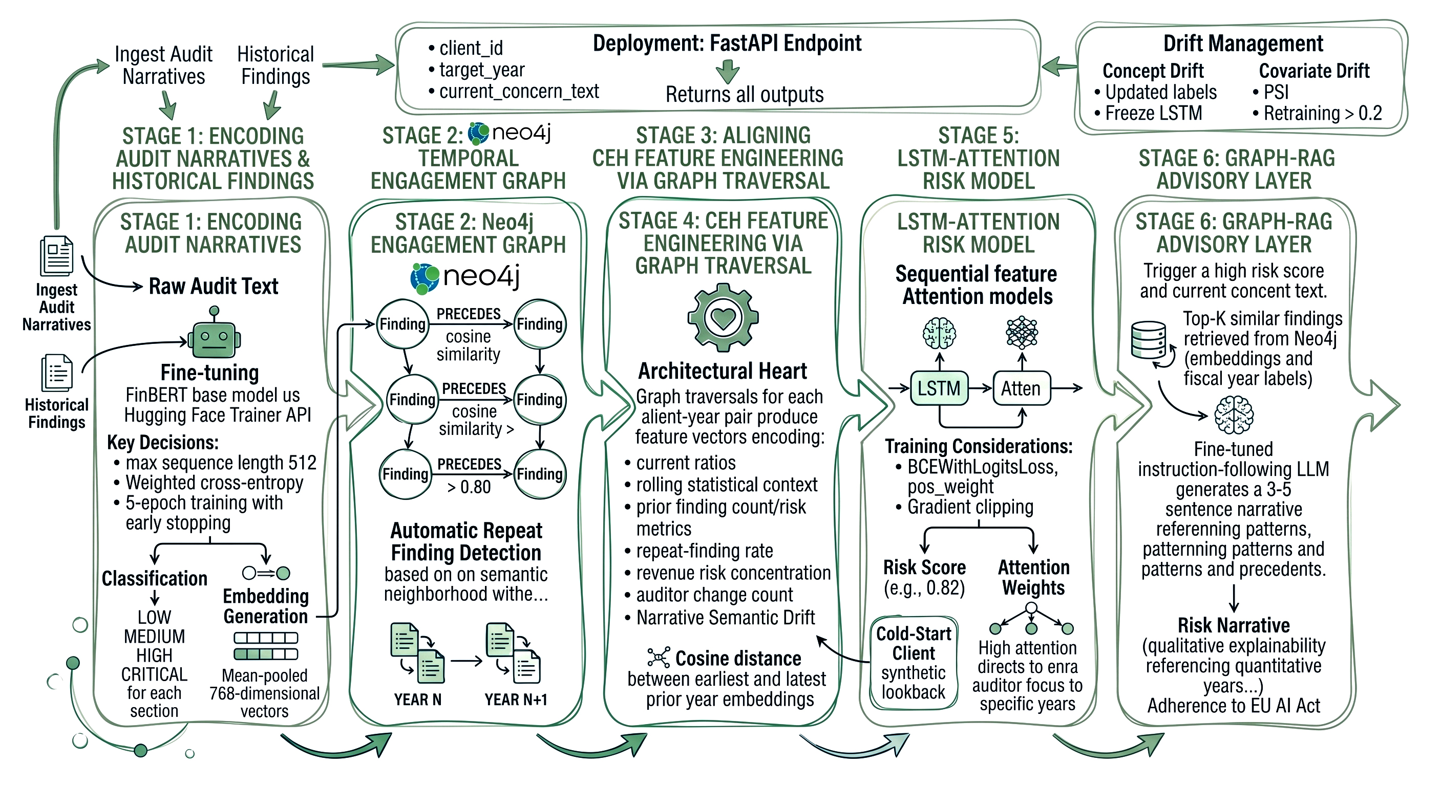
This is the architectural heart of the system. For each client-year pair, a graph traversal produces a feature vector that encodes:
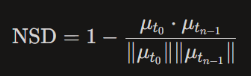
An NSD of 0 indicates that the thematic content of audit findings has remained stable across the full lookback window. An NSD approaching 1 indicates maximal semantic divergence the language, assertion focus, and risk themes present in recent engagements bear little resemblance to those of earlier years. In practice, NSD values above 0.35 have been observed to correlate with significant shifts in control environment characterisation, such as a transition from operational findings to entity-level control concerns. NSD is computed per client-year pair and enters the CEH feature vector as a continuous scalar alongside the financial ratio features.
The narrative_semantic_drift feature deserves special attention because it has no equivalent in ratio-based analysis. A client whose audit narratives have shifted in vocabulary, in assertion focus, in tone from operational findings toward control environment concerns over five years is exhibiting a measurable change in risk profile, even if no single year crossed an outlier threshold. That drift is now a model feature.
The CEH feature vector for each year becomes one timestep in a sequence. The model receives the full sequence of annual feature vectors for a client and learns temporal patterns across them.
import torch import torch.nn as nn import torch.nn.functional as F

class AuditRiskLSTMAttention(nn.Module):

def init(self, input_dim: int, hidden_dim: int = 128, num_layers: int = 2, dropout: float = 0.3):

super().init()

self.lstm = nn.LSTM(input_dim, hidden_dim, num_layers, batch_first=True, dropout=dropout)

self.attention = nn.Linear(hidden_dim, 1)

self.classifier = nn.Sequential(

nn.Linear(hidden_dim, 64), nn.ReLU(),

nn.Dropout(dropout), nn.Linear(64, 1), nn.Sigmoid()

)

def forward(self, x, mask=None):
    lstm_out, _ = self.lstm(x)                        # (B, T, H)
    scores = self.attention(lstm_out)                  # (B, T, 1)
    if mask is not None:
        scores = scores.masked_fill(mask.unsqueeze(-1) == 0, float('-inf'))
    weights = F.softmax(scores, dim=1)                 # (B, T, 1)
    context = (weights * lstm_out).sum(dim=1)          # (B, H)
    return self.classifier(context), weights.squeeze(-1)
Note: Please note that the above are representational code snippets and not production ready.
The model returns two outputs: the risk score (a float between 0 and 1) and a temporally indexed Attribution Map across each year in the engagement sequence. Attribution Maps are not a side product of the attention mechanism they are a primary engineering requirement, designed from the outset to satisfy the explainability obligations that regulators and audit oversight bodies increasingly impose on AI-assisted assurance processes.
In XAI literature, an Attribution Map is defined as a function that assigns a relevance score to each input feature or timestep with respect to the model's output identifying not just what the model predicted but which inputs drove that prediction and by how much. In the CEH context, each entry in the Attribution Map corresponds to a fiscal year in the lookback window. A high attribution score on Year 3 in a 7-year sequence is a precise, auditor-facing statement: "The dominant risk signal contributing to this score originated three years ago." That is not a confidence interval or a black-box probability it is a directional instruction that tells the engagement partner exactly where to focus substantive testing. When an audit committee or regulator asks "why did your model flag this client as HIGH risk?", the Attribution Map provides a structured, year-level answer that can be documented in the working papers and traced back to specific findings in the engagement graph.
Class imbalance is the dominant training challenge in audit datasets genuinely high-risk client-years are rare by design. Using BCEWithLogitsLoss with a pos_weight computed from the training set ratio (negative cases divided by positive cases) corrects for this without requiring oversampling. Gradient clipping at max_norm=1.0 stabilises training on the short sequences typical of audit engagements (3–7 years of history per client).
The retrieval query traverses the engagement graph for the target client, computes cosine similarity between the current-year concern text (provided by the engagement manager) and all prior finding embeddings, and returns the closest matches. Each retrieved finding carries its verified Neo4j node ID a stable, graph-native identifier that uniquely addresses a specific Finding node with a known fiscal_year, risk_level, category, and section_text property set. These node IDs are passed into the LLM prompt as the exclusive evidentiary boundary for generation.
Before the narrative is released to the inference endpoint, it passes through a grounding loop a post-generation verification step that parses every factual claim in the LLM output and checks it against the node properties of the Neo4j IDs supplied in the prompt context. Any sentence that contains an assertion a fiscal year reference, a finding category, a risk level, a management response characterisation is matched against the corresponding node property. Claims that cannot be grounded to a verified node property are flagged and either removed or replaced with a conservative hedge. The grounding loop runs as a deterministic rule-based pass, not a second LLM call, to prevent the verification layer itself from introducing hallucinations.
At the generation layer, constrained decoding enforces that all fiscal year references, finding categories, and risk level labels in the output vocabulary are drawn exclusively from the token set present in the retrieved node properties. This is implemented as a prefix-constrained logit mask applied at each decoding step tokens that represent years, risk labels, or entity names not present in the verified context receive a logit value of −∞, making them impossible to sample. The practical effect is that the model cannot invent a finding from FY2019 if no FY2019 node was retrieved, cannot describe a finding as CRITICAL if its verified node carries a HIGH label, and cannot reference a control category that does not exist in the client's engagement graph. Together, the grounding loop and constrained decoding form a two-barrier hallucination prevention architecture the first barrier operates at generation time through vocabulary restriction, the second operates post-generation through claim verification against graph-native source of truth.
This two-layer explanation quantitative (Attribution Maps identify which years drove the score) and qualitative (Graph-RAG identifies which findings from those years are analogous, with every claim grounded to a verified node ID) directly addresses the explainability and factual accuracy requirements imposed on high-impact AI systems under frameworks including the EU AI Act and the IAASB's emerging guidance on technology-assisted audit procedures.
The full pipeline is served via a FastAPI endpoint that accepts a client_id, target_year, and a free-text current_concern_text from the engagement manager. It returns the risk score, risk tier, top attention years, and the Graph-RAG narrative in a single response. The endpoint loads the fine-tuned BERT embedder, the LSTM-Attention model, and the Neo4j driver at startup using FastAPI's lifespan context manager.
Audit risk models face two distinct drift types that differ from standard ML monitoring:
Regardless of drift type, no retrained model should be promoted directly to production in an audit context. The stakes of a miscalibrated risk score during a live engagement a suppressed CRITICAL flag, an inflated risk tier triggering unnecessary substantive procedures are too consequential to absorb within a single cycle. The recommended transition mechanism is a shadow deployment strategy.
When a retraining trigger is hit whether from concept drift following a standards update or from covariate drift detected via PSI monitoring the updated model is deployed in shadow mode alongside the current production model. Both models receive identical inference requests for the duration of one full audit cycle. The shadow model's outputs are logged, scored against ground truth where available, and compared against the production model across three evaluation dimensions:
Cutover is authorised only when all three dimensions fall within acceptable bounds across the full shadow cycle. This protocol ensures that model transitions are treated with the same change-management rigour applied to any other audit methodology update documented, reviewed, and signed off before the new model touches a live engagement. In enterprise deployments, the shadow cycle naturally aligns with the interim-to-final engagement window, making it operationally invisible to the engagement team while providing a complete real-world validation dataset before promotion.
For new clients with fewer than three years of engagement history, there is insufficient lookback for the LSTM to function meaningfully. The recommended approach is peer-cohort synthetic lookback: retrieve the 10 most structurally similar clients from the graph (matched on industry code, revenue band, and jurisdiction) and inject their rolling CEH features as synthetic prior-year context. The model was trained on a mixture of organic and synthetic sequences, so this does not require a separate inference path it simply populates the earlier timesteps of the input tensor with cohort-derived values rather than client-specific ones.
The distinction is not just technical it is epistemic. Outlier detection asks: "Does this period look unusual compared to the population?" CEH-based risk profiling asks: "Does this period fit a pattern that this specific client has been building toward?"

A Z-score flag on receivables days is noise for a business that restructured its collections policy. The same receivables increase, after traversing a graph that surfaces two prior findings of management override and a going concern note in the prior year narrative, is a critical risk signal. The numbers are the same. What changed is what the system knows about their history.
With the implementation patterns in this second part, the Connected Engagement History is no longer an architectural sketch it is a deployable system. The temporal graph, feature traversals, LSTM Attribution Maps, and Graph-RAG layer together form an audit AI stack that can explain itself, defend its outputs, and evolve under standards changes without destabilising live engagements.
Critically, the controls around the model are as engineered as the model itself. Hallucination is constrained by grounding responses to verified Neo4j node IDs, model updates are throttled through drift monitoring and shadow deployment, and cold-start clients are handled through peer-cohort synthesis rather than silent fallbacks. The system behaves like an audit methodology update: versioned, documented, and reviewable not like an opaque algorithm dropped into the workflow.
This is what it means to move beyond the amnesiac model. Risk assessment becomes a longitudinal, explainable process rooted in institutional memory, not a sequence of cross-sectional anomalies. In that shift, predictive AI stops being a black box bolted on after the fact and becomes an auditable, standards-aligned component of the engagement itself.